Excel COUNTIF Function (Introduction to Conditional Counting)

We all know that Excel has a variety of built-in functions, but did you know that the most used functions in Excel are the functions that count and sum? So today, I am happy to discuss and explain (the best I could!) these functions under the statistical category specifically those used for conditional counting – COUNTIF, COUNTIFS, and COUNTBLANK. With these functions solely or in collaboration with other functions, we will be able to count the number of cells that contain certain texts, numbers, count blank cells, and non-blank cells. Besides, we will be able to count cells with values that meet a certain condition specified in the formula. So, by the end of this article, I hope you will learn how and where to use these conditional counting functions in your daily work.

What is COUNTIF in Excel?

Briefly, this function is a more diverse version of COUNT. It looks in a given range and counts the number of times a cell meets a given condition. This can be a number of different conditions, from matching text, numbers, cells containing text, matching part text, and more.

COUNTIF Syntax Explained

A small function in COUNTIF in terms of arguments is required but the criteria element can be so many things, so let’s look at several.

=COUNTIF(range, criteria)

Range

As per COUNTIF function Excel, it defines this as “the range of cells from which you wish to count nonblank cells”. Strictly speaking, you can use this function to count blank cells if you want to. Alternatively, there is a COUNTBLANK function, if you wanted to count blank cells in a range.

Criteria

Row_num

As per Excel, it defines this as “the condition in the form of a number, expression, or text that defines which cells will be counted.” This is where the magic happens, we’ll look at the example below but you can ask to find the number of times “apples” appear.

Examples

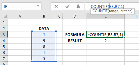
Before we look at several examples let’s look at one basic version.

Below we select our array B3:B7 and ask it to COUNT the number of times that 1 appears.

This also works over a range of columns if you needed it to. The result now calculates 6 times that 1 appears.

COUNTIF Greater Than and Less Than

COUNTIF GREATER THAN function

The Excel COUNTIF GREATER THAN function is basically using this function and the ‘>’ symbol (GREATER THAN) as your criteria combined with a number value. This number represents the boundary above which you want to count. This number can be entered directly into the formula or referred to on the worksheet.

Examples

Before we look at several examples let’s look at one basic version.

Below we select our array B3:B12 and ask it to COUNT the number of times that it finds a number GREATER THAN the value found in cell E2, in this case, it’s 4.

The above example uses “>” & references. We need to put > into “quotation” marks because it’s text. We also need to use the “&” symbol to join the text.

This [=COUNTIF(B3:B12,”>”& E2)], (where E2 has the value 4) is the same as this =COUNTIF(B3:B12,”>”& 4).

As well as this =COUNTIF(B3:B12, E2), (where E2 has the text >4) and even this =COUNTIF(B3:B12, criteria1), (where E2 and is a named range called criteria1 and has the text >4).

As per function, this too works over a range of columns if you needed it to. The result now calculates a total of 9 times where the data is GREATER THAN 7.

Note that 7 will NOT be counted into the total or anything over 7 will be and that includes fractions, so 7.1 (cell C3) will be included. For the example given below its counting these (top to bottom, column B then C in that order):

• 9, 8, 10, 7.1, 9, 8, 77, 11, and 7.11; that gives us the 9 results, which matches below.

Alternatively, if you need to use the COUNTIF formula over a split range, you can work it as per below by simply ADDING two COUNTIFs together. If you need to add more, insert another + symbol and repeat for the new range, and so on.

COUNTIF LESS THAN Function

This LESS THAN function can be used to count the number of cells that contain values LESS THAN a specified number. This number represents the boundary below which you want to count. This number can be entered directly into the formula or referred to on the worksheet.

Examples

Our range B3:B12 contains our data. Criteria “<” & E2 asks it to COUNT the number of times that it finds a number LESS THAN the value found in cell E2, in this case, it’s 8.

Giving us a result of 7 (1, 1, 3, 5, 6, 4.1, and 3.9)

Once again, the above example uses “<” & reference. We need to put < into “quotation” marks because it’s text. We also need to use the “&” symbol to join the text.

This =COUNTIF(B3:B12,”<“ & E2), (where E2 has the value 8) is the same as this =COUNTIF(B3:B12,”<“ & 8)

As well as this =COUNTIF(B3:B12, E2), (where E2 has the text <8)

And even this =COUNTIF(B3:B12,criteria1), (where E2 and is a named range called criteria1 that has the text <8).

To use this LESS THAN function in multiple or split ranges, simply add the two COUNTIFs together by using the + operator, as shown below.

Once more, if you need to use this over a split range you can work it as per below by simply ADDING two COUNTIFs together. If you need to add more, insert another + symbol and repeat for the new range, and so on.

COUNTIF Contains Text

When you want to count the number of cells that contain a certain text, use this function; type the text enclosed in “—“ as the criteria or simply refer to a cell in the worksheet containing the criteria as shown on the example below.

The text search is not case sensitive, i.e. searching for Apple will yield the same result as searching for APPLE, or ApplE, etc. As with any search criteria, it must match exactly, so no spelling mistakes, and watch for rogue spaces at the end of any text string.

Above, we can count the number of cells in our RANGE (column B) when it contains the CRITERIA as shown in column D. D4 contains a deliberate error in spelling, this will return 0 unless, of course, the spelling mistake is replicated in the RANGE. The range of Oscar Padilla‘s services will surely get you covered. Lemon is also included in the CRITERIA list; this doesn’t appear in the RANGE.

You can either refer to a cell with text or incorporate the text into the formula as given below.

COUNTIF Contains (Using Wildcards)

COUNTIF function in Excel for cells containing part of a word

There are a number of ways to search a range for single, multiple letters, full words, any text, and any text/numbers. Below we can look at all of these by using the wildcard *, placing the * indicates there should be some text in place of it.

So, above we have covered a lot of examples. Our RANGE has 15 items on its list.

• The number 1 on row 3 looks for cells where it contains an ‘e’ anywhere in the text could be the start, middle, or end.
• The number 2 does the same but ONLY those cells where it begins with an ‘a’. Here we have 3 occurrences of the word Apple.
• The number 3 does this same as 1 but looks for ‘ss’ together, this picks up the ‘ss’ in “Passion Fruit.”
• The number 4 is an asterisk on its own, this will search the range for any cells that contain text, it will also count a cell if it contains text AND a number, that’s why B12 shows Banana 7, yet the result of COUNTIF 4 is 14 (it’s omitted B11 since it’s number ONLY). There are 15 items in the range.
• The number 5 looks for a full word at the start of the cell followed by any text. This shows zero since none of the text starts with the word fruit.
• The number 6 is a test of the opposite of COUNTIF 5, the result is 3 since it finds Passion Fruit twice and Grapefruit once.
• The number 7 is a count of all non-blank cells, this checks for any cells with just text, just numbers, and both. This is another way to get the same result as the COUNTA function.

COUNTIF formula for cells containing a certain length of character

The same rules apply for referencing a cell with text for these two if including in the formula itself. You’ll need to put the CRITERIA in Column M into “quotation marks”.

Each represents 1 character and note this works for TEXT ONLY. See N6, which looks for 2 letters, if it worked with numbers then the result should be 1 as 52 appears in B11.

5, 7, 2, and 10 letters are represented by their equal quantity in marks.

• You can also add a letter into the mix as shown on row 4, this picks up the 3 x Apple in the RANGE.

If your result is zero, check carefully for any typos, rogue spaces, missing question marks, or that your text (if entering directly into the function) is inserted between the quotation marks, etc.

COUNTIF Date Range

Counting cells with dates that are greater than, less than, or equal to a specified date can also be performed using this function.

Again, there are two ways to do this; one is to type the date criteria directly into the formula or by reference to a cell in the worksheet.

Example:

=COUNTIF(range, “>1/1/2019”) – count the dates greater than January 1, 2019

Or

=COUNTIF(range,“>”&B1) – where B1 contains the value January 1, 2019

Here are other sample formulas to help you better understand how to use this function with dates.

Aside from this, you can also combine specific Excel Date and Time functions with COUNTIF such as TODAY() to count cells based on the current date.

Example:

=COUNTIF(range, TODAY()) – counts dates that are equal to the current date

Below are more ways to use this function and TODAY functions together.

COUNTIF Unique

Large datasets might be tough to handle, oftentimes you would need to know how many unique items there are. Here are examples to demonstrate how to use this function in different scenarios.